CS180 Project 2 - Fun with Filters and Frequencies

Introduction

In this project, we explore the use of filters and frequencies in image processing. The project is divided into two parts where we work with gradient magnitude computation, unsharp masking, hybrid images, and multiresolution blending. Each section details the process and provides visualizations to demonstrate the results. I would say that the most interesting thing that I learned from the project as a whole is how to use low and high pass filters to get different effects on the human eye from photos. I didn't really have any signal processing experience before this class.

Gradient Magnitude Computation

We compute the gradient magnitude of an image to detect edges. The reason why we are able to do this is because the gradient magnitude of the image corresponds to the intensity of the greatest change in the image. This is useful for edge detection because edges are where the intensity of the image changes the most. The magnitude is calculated by taking the square root of the sum of squared partial derivatives Gx and Gy, which correspond to the directional changes in the horizontal and vertical directions respectively. My specific approach was as follows: A finite difference kernel was created for the x and y partial derivatives using np.array([[1, -1]]) for x and np.array([[1], [-1]]) for y. These kernels were applied to the image using scipy.signal.convolve2d to compute the partial derivatives in each direction. The gradient magnitude was then calculated by combining these derivatives using np.sqrt(dx_deriv ** 2 + dy_deriv ** 2), effectively taking the L2 norm of the gradient vector at each pixel to produce the final edge image. Below is an example of the computed gradient magnitude of the cameraman image, shown split into its x and y components before being combined:

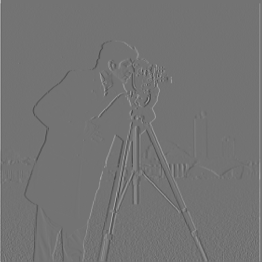
Finite Difference Operator (X)

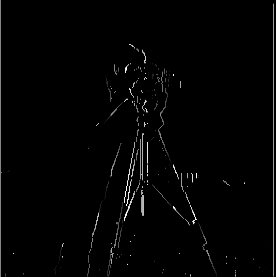
Binarized Finite Difference Operator (X)

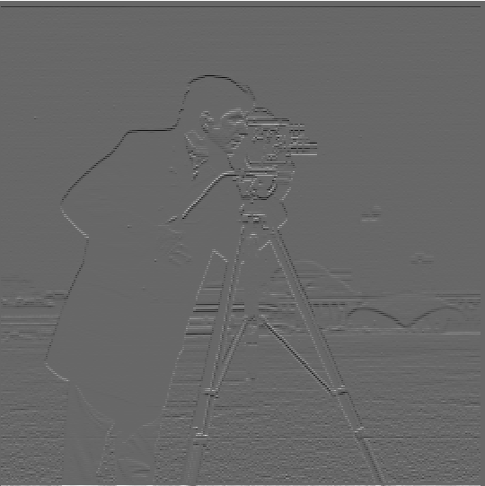
Finite Difference Operator (Y)

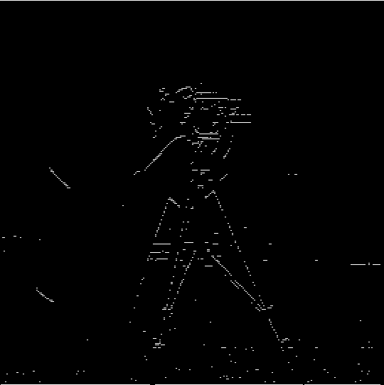
Binarized Finite Difference Operator (Y)

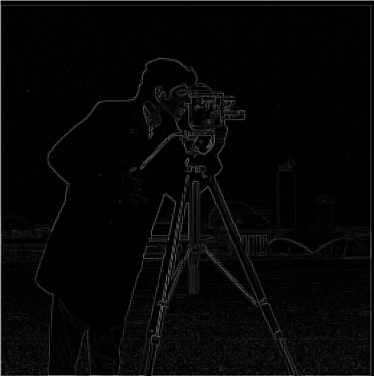
Gradient Magnitude

Binarized Gradient Magnitude

Gaussian Blurred Finite Difference

With this approach, we first blur the original image using a Gaussian filter. I made sure to choose an appropriate kernel size and standard deviation (10, 1) and then I performed the same operation as earlier on the now blurred image. Overall, I noticed in this case that the Gaussian filter was able to smooth out the image and reduce the noise, which made the edges more pronounced and rounded. This is because the Gaussian filter is a low-pass filter that removes high-frequency noise from the image. In addition, certain fine details of the image were lost as a result of the blurring, so there's a clear trade off. The results are shown below.

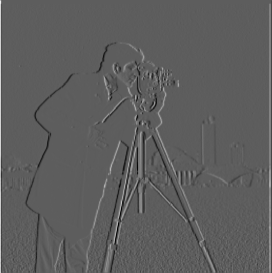
Blurred (X)

Binarized Blurred (X)

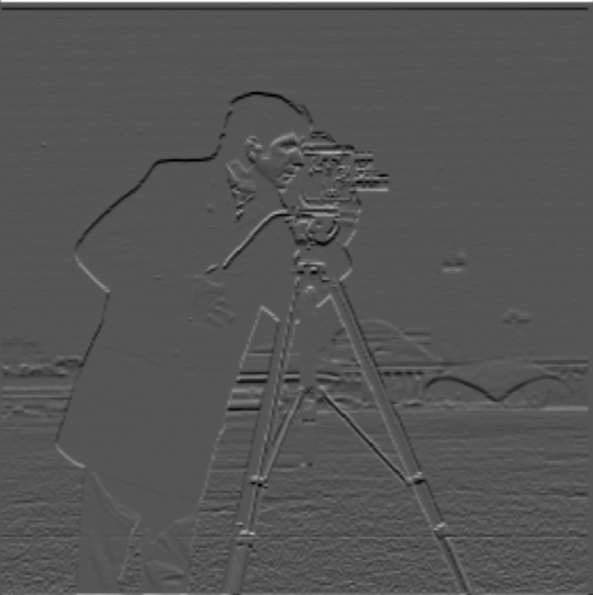
Blurred (Y)

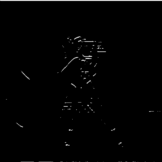
Binarized Blurred (Y)

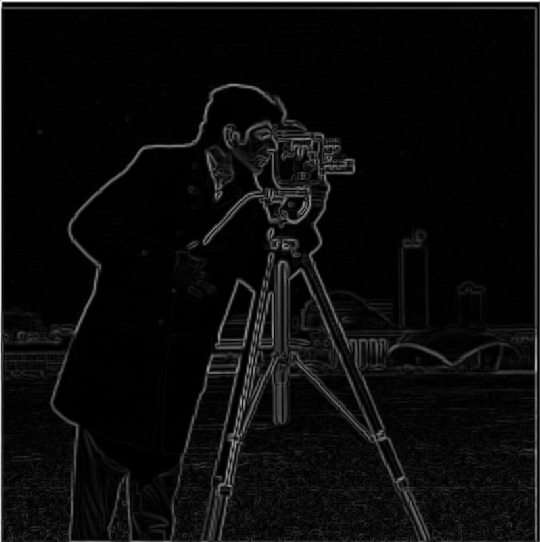
Blurred Gradient Magnitude

Binarized Blurred Gradient Magnitude

Derivative of Gaussian (DOG)

This has the same result as blurring the original image with the Gaussian filter, but it only requires one convolution. To do this, we simply convolve the Gaussian with dx and dy and then apply the filter. Results are shown below, and are nearly identical to the previous section

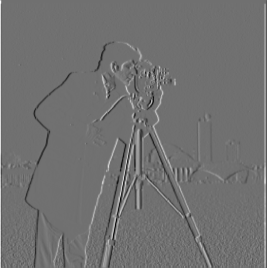
DoG (X)

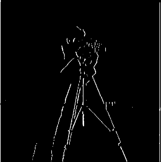
Binarized DoG (X)

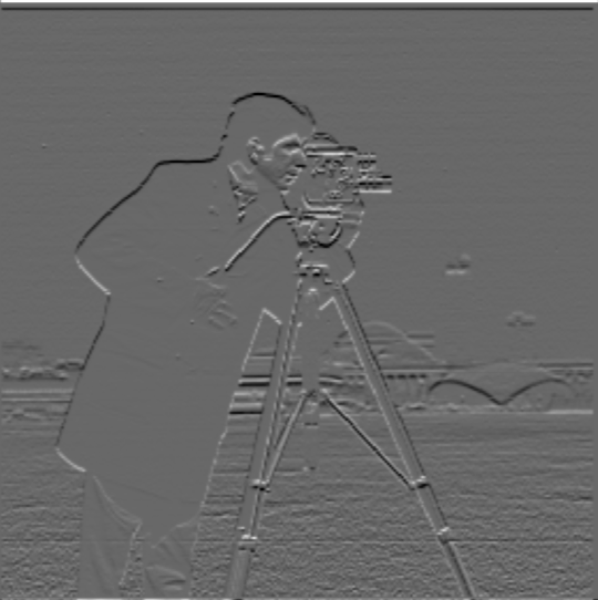
DoG (Y)

Binarized DoG (Y)

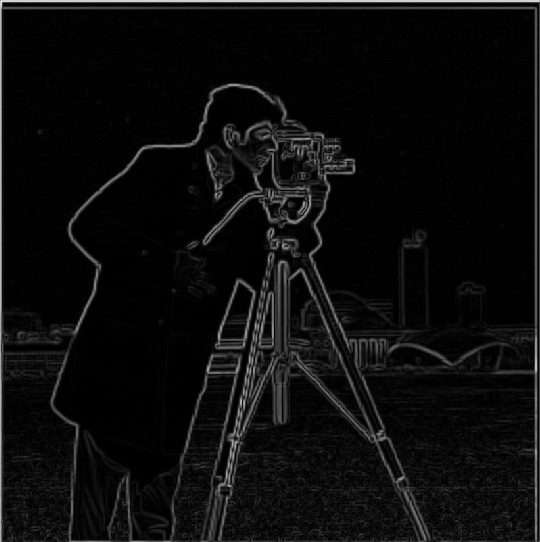
DoG Gradient Magnitude

Binarized DoG Gradient Magnitude

Unsharp Masking

Unsharp masking is a technique used to sharpen an image by emphasizing its high-frequency components. Below, you can see the progression from the original image to the sharpened image from Alpha 2 to 4:

Original Taj Mahal

Sharpened Taj Mahal (alpha = 2)

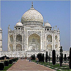
Sharpened Taj Mahal (alpha = 3)

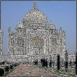
Sharpened Taj Mahal (alpha = 4)

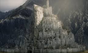
Original Minas Tirith

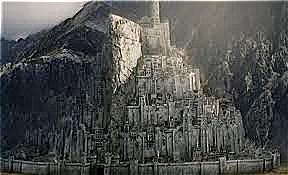
Sharpened Minas Tirith (alpha = 2)

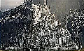
Sharpened Minas Tirith (alpha = 3)

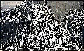
Sharpened Minas Tirith (alpha = 4)

Below, we show the result of taking an already sharpened image, the one ring, blurring it, and resharpening. In this case, you can see that the ring's text is much more pronounced and the edges of the map of middle earth are much sharper.

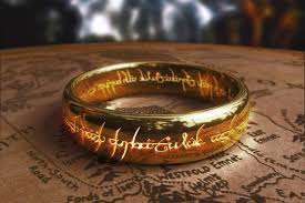
Original One Ring

Blurred One Ring

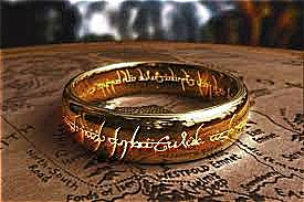
Resharpened One Ring

Hybrid Images and Fourier Analysis

Hybrid images are created by blending high frequencies from one image with low frequencies from another. I show two successful examples and one less successful attempt. Below are examples of hybrid images along with their Fourier analysis:

Nutmeg

Derek

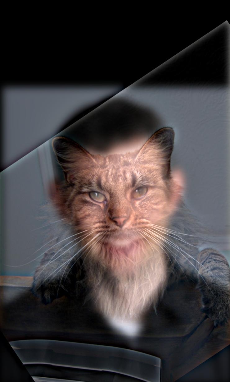
Derek + Nutmeg

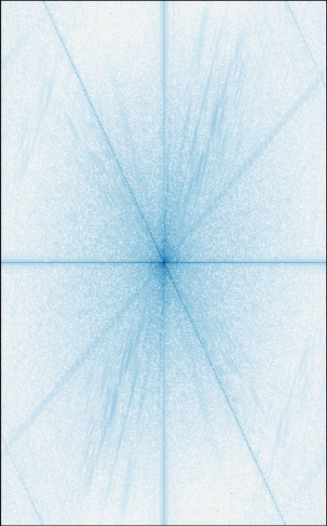
Fourier Analysis of Original Nutmeg

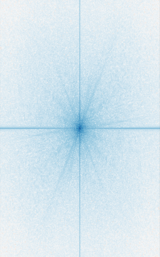
Fourier Analysis of Original Derek

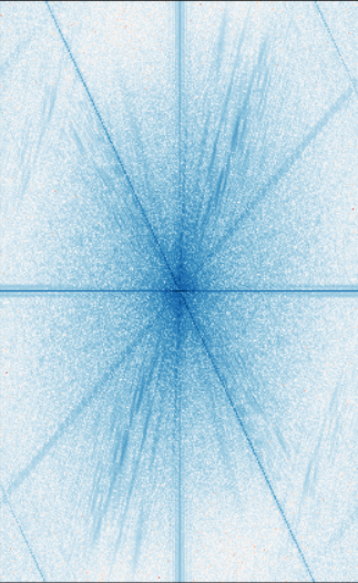
Fourier Analysis of High pass filtered Nutmeg

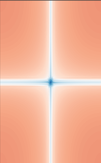
Fourier Analysis of Low pass filtered Derek

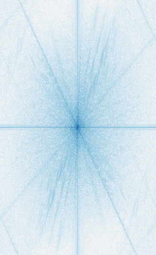
Fourier Analysis of Hybrid Combined Image

Here is one more example of a successful blend of images, namely Gumbledore from combining Gimli and Dumbledore

Gimli

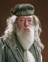
Dumbledore

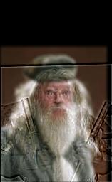
Gumbledore (Gimli + Dumbledore)

It seems like I couldn't get a good hybrid for these pictures of Bilbo Baggins and Legolas from LoTR. This is a failed example that didn't turn out great.

Bilbo

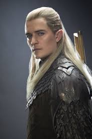
Legolas

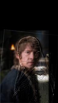
Bilbolas (Bilbo + Legolas) (Failed Example)

Multiresolution Blending and Gaussian / Laplacian Stacks

In this process, the Gaussian stack is created by applying a Gaussian blur to each level without downsampling, so the image size remains consistent across all levels. The Laplacian stack is computed by subtracting consecutive levels of the Gaussian stack to capture edge-like details at different scales. Specifically, each level of the Laplacian stack is obtained by subtracting the next level of the Gaussian stack from the current level. Below, you can see the result of the gaussian stacks at different depth when applied to the apple and orange images.

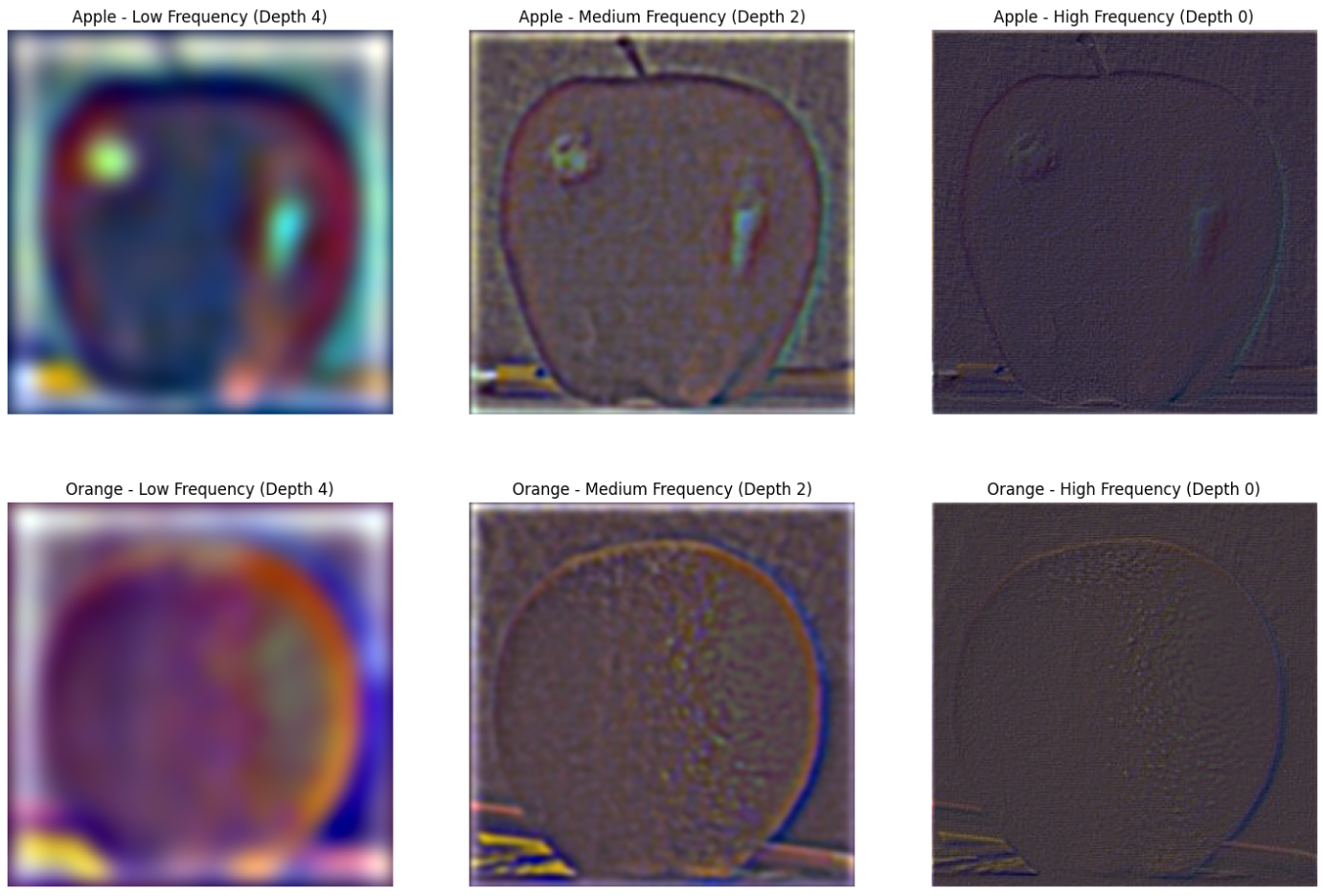
Gaussian Stack Visualization

Multiresolution blending allows us to seamlessly blend two images together. Below, the two original images are shown on the left and right, with the blended image in the center:

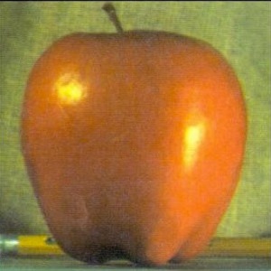
Original Apple Image

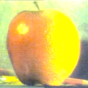
Blended Orapple (Apple + Orange)

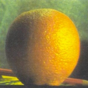
Original Orange Image

Though the final result is shown above, here is a progression of the mask and the blended result at each layer of the stack

Original Mask (Depth 0)

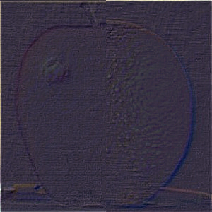
Blended Layer 0

Original Mask (Depth 2)

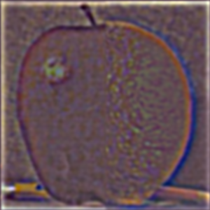
Blended Layer 2

Original Mask (Depth 4)

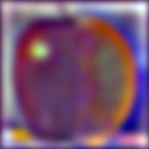
Blended Layer 4

Here is an example of a mountainous sunset and a beach sunrise blended together with a horizontal mask

Original Sunset Image

Original Sunrise Image

Blended Sunset/Sunrise

Horizontal Mask Used for Sunset/Sunrise

Below is an example of multiresolution blending with an irregular mask (Barad-Dur + Windows XP Background):

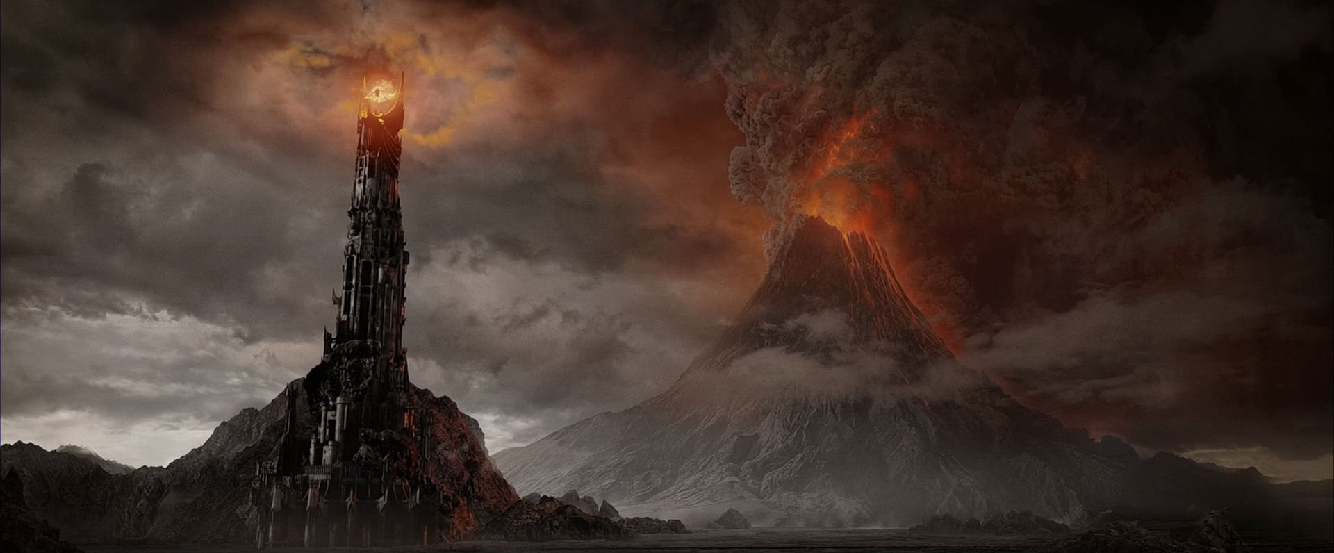
Original Barad-Dur Image

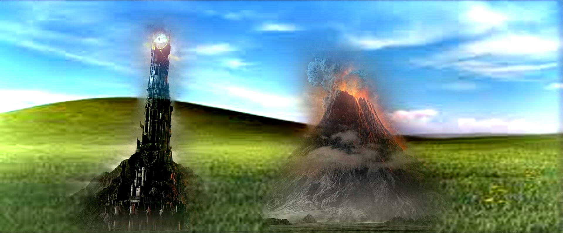
Baraddows XP (Barad-Dur/Mount Doom + Windows XP Background)

Original Windows XP Image

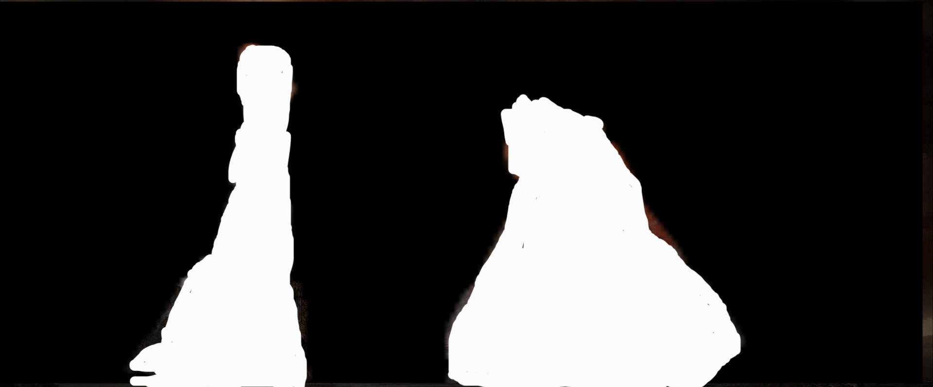
Irregular Mask Used for Barad-Dur/Mt Doom